
This post is a first a series that I called "From Stata to R". If you also like to pass from one software to the other depending on the things you want to do (and the time you have), I figured this series of posts could help out.
This one shares some codes that allow plotting the predicted effect of an interaction term in 3D, by saving the coefficients in Stata and plotting them in R such as
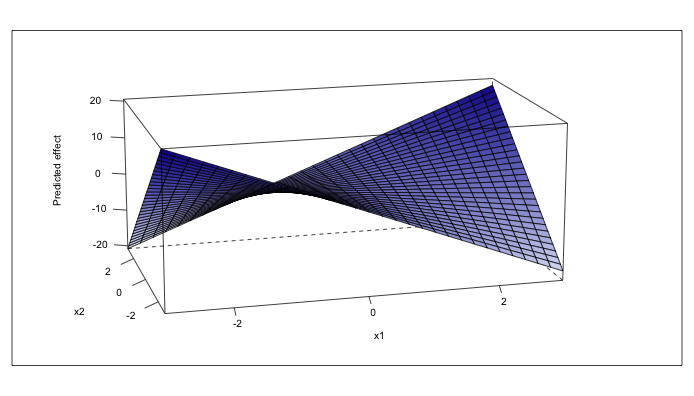
If you have a model of the type: y = a + b1*x1 + b2*x2 + b3*x1*x2 + u, and you would like to plot their total effect (not only the marginal effect of one or the other), you can use Stata to estimate the coefficients and save them; R then comes in to 3D plot the predicted effect. All the sources files (do, R and data) as well as the plot have been posted on Github.
In Stata:
// CHANGE DIRECTORY to reflect yours
cd "/Users/oliviadaoust/GitHub/From-Stata-to-R"

set more off

drop _all
clear
set obs 500

set seed 10101

**** generates three normally distributed variables N(0,1)
gen x1 = invnormal(runiform())
gen x2 = invnormal(runiform())
gen u = invnormal(runiform())

**** sum stats (to be used for the 3D plot range)
sum x1 x2

**** generates interaction
gen x1x2 = x1*x2

**** y = xB + u
gen y = 0.04*x1 - 0.4*x2 + 2.2*x1x2 + u

**** regression
xi: reg y x1 x2 x1x2

**** save coefficients
matrix b = e(b)

**** restricting to the three coefficient needed
mat coef = b[1,1..3]
mat list coef // displays [coef]

**** transforms the matrix into a dataset
matsave coef, dropall replace

**** save as dataset
saveold "coef.dta", replace
In R:
library(lattice)
library(colorspace)
library(foreign)

## change to your directory
setwd("/Users/oliviadaoust/GitHub/From-Stata-to-R/")

## opens the file containing coefficients estimates saved in Stata
coef <- read.dta("coef.dta")
coef

## generate data points (from summary statistics)
data = data.frame(
x1 = rep( seq(-3, 3, by = 0.2), 60),
x2 = rep( seq(-3, 3, by = 0.2), each=60))

## estimate effect of the coefficient of interest and their interaction
data$x1x2 = (data$x1*coef[,2] + data$x2* coef[,3] + coef[,4] * (data$x1*data$x2))
#coefx1 is the coefficient associated to x1, etc.

## range of colors
newcols <- colorRampPalette(c("aliceblue", "darkblue"))

## 3D plot
wireframe(x1x2 ~ x1 * x2, data=data,screen=list(y=0, z=15,x=-75) ,
aspect = c(0.55,0.4),panel.aspect=0.5,drape = TRUE,col.regions = newcols(100),colorkey=F,
xlab = list("x1",cex=0.85), ylab = list("x2",cex=0.85),
zlab = list("Predicted effect",rot=90,cex=0.85),
scales=list(arrows=FALSE,cex=0.85,tick.number=4, col="black"))